Foucault pendulum simulation

Picture 1. Image
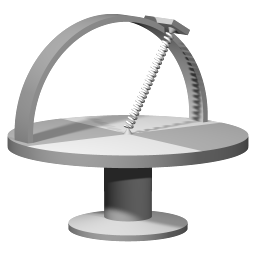
Wheatstone's design that displays the same effect as the Foucault pendulum.
Transcript of Wheatstone's describing note

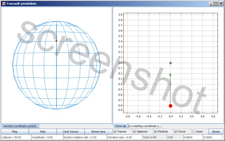
The sphere represents the rotating Earth. The grey dot represents the suspension point of a pendulum. The red dot represents the pendulum bob. The green arrow represent the force towards the point of suspension. More precisely, the green arrow represents the force component parallel to the local surface.

In this simulation the pendulum bob is confined to motion along the surface of the sphere. That way a coordinate system with two spatial degrees of freedom can be used: spherical coordinates with a fixed radial distance. The calculation is only approximative, but the accuracy suffices: the simulation predicts the Foucault effect just as it is observed in actual Foucault pendulum experiments.

Besides the Foucault pendulum itself there are other setups that display the Foucault effect. Image 1 represents a tabletop device that Wheatstone constructed in 1851, that succesfully reproduced the Foucault effect. Links to other descriptions of tabletop devices displaying the Foucault effect are presented in the Foucault pendulum article.

Picture 2. Image.
- Blue arrow: gravity, acting towards the center of gravitational attraction
- Red arrow: the force that the pendulum wire exerts on the pendulum bob.
- Green arrow: the resultant force of gravity and the wire tension.

Evolution of the simulation

A Foucault pendulum that isn't swinging is effectively a plumb line, and a plumb line hangs perpendicular to the local (level) surface. Picture 2 illustrates why this is the case. Due to its rotation the Earth has an equatorial bulge. A plumb line does not point exactly in the direction of the Earth's center of gravitational attraction: there is an angle between the force towards the center of gravitational attraction and the force that the pendulum wire exerts on the bob. On Earth, at 45 degrees latitude, that angle is about a tenth of a degree. In the case of the world's largest Foucault pendulum, the one in the Pantheon, with a 67 meter long wire, that amounts to a displacement of the pendulum bob of about 10 centimeters.

Picture 2 illustrates that the resultant force of gravity and wire tension provides the required centripetal force. The shape of the Earth is an equilibrium shape; the Earth's shape matches its rotation rate. The Earth's equatorial bulge and a plumb line's displacement have the same origin: the necessity to provide required centripetal force. That is why at every latitude a plumb line hangs perfectly perpendicular to the local surface.

When the pendulum is swinging the midpoint of the swing is the displaced point. The default setting of the simulation has the pendulum swinging with a very small amplitude, about as large as the displacement, but the simulation controls allow you to explore other amplitudes.

Effects during each halfswing

The pendulum bob is circumnavigating the Earth's axis. During a swing towards the Earth's axis the pendulum bob gains angular velocity, so it turns to the right, and during a swing away from the central axis of rotation the pendulum bob loses angular velocity, once again turning to the right.

I will call swings parallel to the latitude lines 'forward' and 'backward' swing. (A forward swing is when the pendulum bob swings to the East, a backward swing is when it swings to the West.) During forward and backward swing the centripetal force that the pendulum bob is subject to is especially significant. During a backward swing the pendulum bob is circumnavigating the Earth's axis slower than the Earth itself. The attracting force is the amount that is required for co-rotating, hence during a backward swing the pendulum bob experiences a surplus of centripetal force. This surplus pulls the pendulum bob closer to the central axis of rotation. This is valid for any amplitude of the pendulum swing. No matter what the pendulum amplitude is, 10 times or a 100 times the displacement, during backward swing the pendulum bob is pulled closer to the Earth's axis.

Finally, during a forward swing there is not enough centripetal force, and the pendulum bob swings wide.

Picture 3. Image
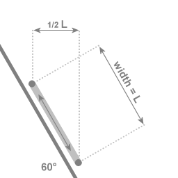
In the case of an angle of 60 degrees with the central axis of rotation: If the two extremal points of the swing are a distance of L apart, then the motion towards and away from the central axis covers a distance of 1/2 L

Dependency on the latitude

On midlatitudes the motion away and towards the central axis of rotation is reduced, and the amount of work that the centripetal force does is proportional to the motion towards and away from the central axis of rotation. As the diagram shows, at 30 degrees latitude the work that is done by the centripetal force is halved as compared to the strictly 2-dimensional case. The reduction is proportional to the sine of the latitude. Less work done means it takes longer to complete a precession cycle. At 30 degrees latitude the precession cycle takes twice as long: 2 full rotations of the rotating system. The period of the precession cycle is the system rotation rate divided by the sine of the latitude.

The simulation's controls

There are six input fields. The first four are for the dynamics of the simulation, the last two are for the view.

• Latitude. The latitude of the attraction point in degrees. If you change the latitude then the field next to the 'turns' field will change also, showing the expected period to complete a precession cycle. You can enter a latitude very close to the poles but then you need to combine that with a very small amplitude to get accurate results.


• Amplitude. The distance of the pendulum bob to the point of attraction at the start of the simulation run.


• System rotation rate. The default setting is 0.5. You can enter a higher value but then there will be too few vibrations for each rotation cycle. You can explore using a very slow system rotation, to get many vibrations to each rotation cycle.


• Vibration rate. The default setting is 4.0; four vibrations per unit of time. You can enter a higher value, but if you use too high a value the calculation will not produce accurate results.

The two input fields for the view:

Zoom. The zoom for the close-up view is automatically adjusted to give a good view, you can adjust the zoom factor with this input field.

Zoom shift. For shifting the close-up view.

When you start altering a value in an input field the field turns yellow. As long as the field is still yellow the input process is not ready. The input is finalized by pressing the Enter key on the keyboard, and then the field will no longer be yellow.

Comparison with actual Foucault pendulums

In the default settings of the simulation the displacement the shift of the midpoint of the swing is about as large as the swing itself. In an actual Foucault pendulum setup the angle of the swing will generally be fifty to a hundred times larger than the displacement.

Method of computation

I discuss the mathematical setup of the Foucault pendulum simulation in a separate article: Foucault pendulum mathematics.

The method of computation is numerical analysis: the trajectory of the particle is calculated by evaluating differential equations.

This simulation has been created with EJS
EJS stores the specifications of a simulation in a plain text file, with extension .xml
You can examine how the simulation has been set up by opening the simulation .xml file with EJS.
Download location for the EJS software
Download location for the Foucault pendulum source file
(The file is zipped because a browser will attempt to parse any .xml file.)

Also available for download: a standalone version of the Foucault pendulum applet (requiring the Java Runtime Environment but not a browser to run)

Text, images and animations are licensed under a Creative Commons Attribution-ShareAlike 2.5 License.

Last time this page was modified: July 17 2010