The calculations in the Foucault rod simulation

This page accompanies the page with the Foucault rod simulation. Here I discuss the way that the calculations have been set up.

The coordinate system is cartesian coordinates.

The three spatial degrees of freedom are the x, y and z direction. In each of these directions the force upon the pendulum bob is decomposed in two components:

An elastic force that arises when the rod is elongated or shortened. In the equations this factor is referred as 'rod length constraining acceleration': a_rlc. In a preliminary calculation step the instantaneous length is evaluated (using Pythagoras' theorem) and the length-at-rest is subtracted from that, giving the deviation from rest length. The factor a_rlc is proportional to that difference, so it's a function of the instantaneous length. a_rlc is made so large that effectively the rod length is fixed; variations in rod length are too small to affect the swinging motion.
An elastic force that sustains a swinging motion of the rod. The period of the swing is ψ . To a good approximation the swing is a harmonic oscillation, so to obtain the acceleration the displacement is multiplied with ψ ².

The rod base is the point where the rod is attached to the support. In the simulation view the rod support is the L-shaped structure that circumnavigates the central axis. Therefore both x_rodbase(t) and y_rodbase(t) are functions of time. In the calculations the x- and y-position are calculated with sines and cosines.

The attraction point is the position where the bob would be if the rod would be in a straight position. The rod resists bending, giving rise to a force towards the attraction point. (Arguably the attraction point could also be called the equilibrium point; when the rod is straight it is in equilibrium. Anyway, the name doesn't matter. In the case of a gravity pendulum the equilibrium point is an attraction point, and I have opted to retain that name.)

Note that the z-position is not a fucntion of time. The system is circumnavigating the z-axis, so the z-position is a constant.

l	The instantaneous length of the rod.
a_rlc(l)	Rod length constraining acceleration as a function of the instantaneous rod length.
ψ	The pendulum's oscillation rate.
rodbase(t)	position of the rod base as a function of time.
attract(t)	position of the attraction point as a function of time.

The values obtained with the preliminiary calculations are subsequently evaluated with the following set of differential equations:

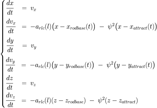
$\begin{cases} \cfrac{dx}{dt} & = \; v_x \\ \cfrac{dv_x}{dt} & = \; - a_{rlc}(l) \big( x - x_{rodbase}(t)\big) \; - \; \psi^2 \big( x - x_{attract}(t) \big) \\ \cfrac{dy}{dt} & = \; v_y \\ \cfrac{dv_y}{dt} & = \; - a_{rlc}(l) \big(y - y_{rodbase}(t) \big) \; - \; \psi^2 \big( y - y_{attract}(t) \big) \\ \cfrac{dz}{dt} & = \; v_z \\ \cfrac{dv_z}{dt} & = \; - a_{rlc}(l) (z - z_{rodbase}) \; - \; \psi^2(z - z_{attract}) \\ \end{cases}$

Because of the algorithm that EJS uses the differential equations must be declared in the above form, with first derivatives but no second derivatives.

Note that there is no explicit centripetal force in these motion equations. The required centripetal force arises automatically from the elasticity of the rod. When the system is rotating the midpoint of the swing is displaced outward. The resistance of the rod to the outward bending provides the required centripetal force.

The effort to keep the length of the rod fixed leads to a number of problems.
In the other Foucault simulation on this site the constraint is incorporated into the very coordinate system. That simulation uses spherical coordinates, and the motion is simply confined to the surface of a sphere. However, in the case of the Foucault rod using spherical coordinate was not an option because the rod is pointing inward, and the bob does not follow the surface of a sphere.

What inevitably happens in the simulation is that the force that constrains the rod length sustains a vibration (This simulation doesn't incorporate friction, so any initial vibration remains forever) This vibration has a much higher frequency than the pendulum swing, and its effect on the pendulum swing is negligable. However, this high frequency means that the numerical analysis must proceed in very small time increments. For every cycle of the lengthwise vibration there must at least 10 time steps. If the time steps are too large the calculation becomes unstable.

The problem of keeping the rod length fixed means that the simulation has to calculcate many more steps than are displayed. In the current version the time increment is 0.005 second, 20 steps between each displayed frame, 10 frames per second.

This work is licensed under a Creative Commons Attribution-ShareAlike 3.0 Unported License.

Last time this page was modified: August 10 2010