This article is part of a set of three; the common factor is Calculus of Variations. In classical physics Calculus of Variations is applied in three areas: Optics, Statics, and Dynamics. Discussion of application in statics is included in this 'Foundation' article.
The other two articles:
| Optics: | Fermat's stationary time | |
| Dynamics: | The Energy-Position Equation |
Overview of the basics of Calculus of Variations, as applied in physics
1 Motivating example
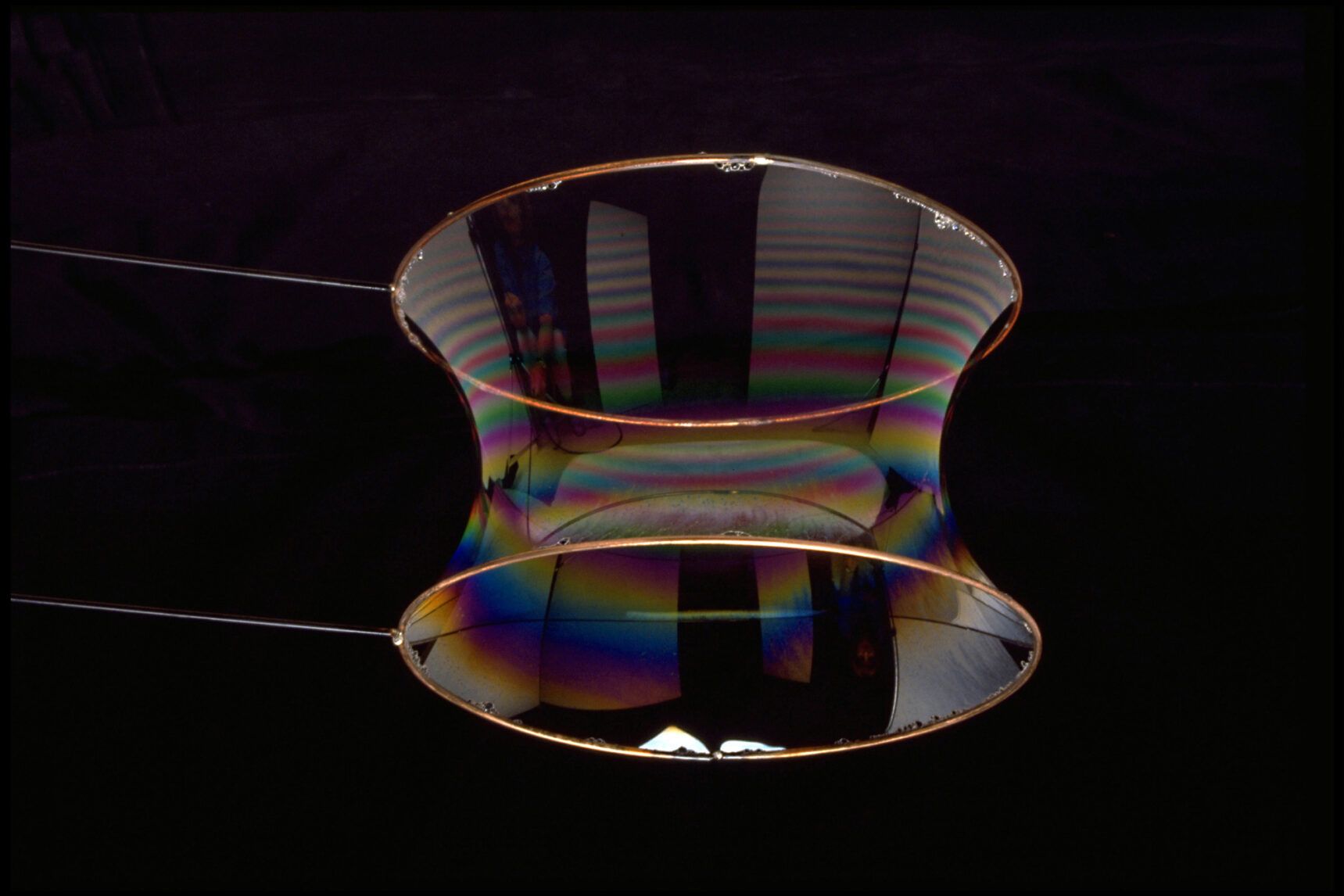
Image credit: Susan Schwartzenberg - Exploratorium
As motivating example for developing Calculus of Variations we will take the case of a soap film that stretches between two co-axial rings, as shown in the image.
The shape of the soap film is a minimal surface. The equation for that shape will be derived using a form of differential calculus.
The strategy:
The surface from ring to ring is a surface of revolution, so we can treat the problem as a two-dimensional problem. Approximate the continuous surface in the form of a stack of truncated cones. In the limit of making those truncated cones infinitesimally thin the resultant surface converges onto the solution to the problem.
Overview:
Section 2 works towards graphlet 2.5, an interactive diagram for the purpose of demonstrating what it takes to solve the minimal surface problem.
Section 3 opens with presenting an economic way of constructing a general differential equation for solving variational problems (section 3.1). Section 3.2 offers a discussion of the method of deriving the Euler-Lagrange equation that the majority of sources offer.
Section 4 Instead of immediately proceeding to apply the Euler-Lagrange equation the discussion moves to a problem related to the soap film: the catenary problem. The catenary problem and the soap film problem are siblings; they have the same solution.
The reason for expanding the discussion to the catenary problem: the catenary problem is particularly well suited to demonstrate how differential calculus and calculus of variations are connected. The catenary problem is first solved with differential calculus and then with application of calculus of variations, with emphasis on the connection. Solving the catenary problem also solves the soap film problem since the two problems have the same Lagrangian.
Section 5 gives the key points from the full discussion of Hamilton's stationary action that is available in an article of its own.
2 Simplest case: two truncated cones
In preperation for later use:
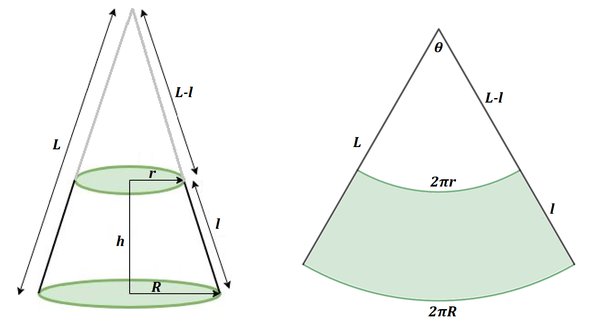
Image credit: Elaine Dawe - Quora
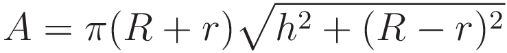
The lateral area of a truncated cone is given by the following expression:
We start with exploration of the simplest case that is an instance of the type of problem that we want to solve:
The surface of a cone is a surface of revolution. So we can use an xy-coordinate system, with the y-coordinate representing the radial distance. Graphlet 2.2 shows 2 cones, projected onto the xy-plane.
The three numbers underneath display the following:
- area of the cone marked '1'
- total area of the two conical surfaces
- area of the cone marked '2'
Moving the slider changes the circumference of the circle where the two cones are adjoined. The value displayed in the slider knob is the radius of that circle
For each cone: the area is a function of the radius in two ways:
- The area is proportional to the circumference
- The area is proportional to the width.
About the width: the steeper the slope, the larger the width. That is: the width is a function of the derivative of the curve.
In graphlet 2.3 the right hand panel gives a overview of how the areas of the two cones respond to sweeping out variation. I will refer to the point where the total surface area is minimal as 'the sweet spot'. As you are sweeping out variation: A1 and A2 are changing in opposite direction. At the sweet spot the two are changing at the same rate.
The curve '-A2' is the mirrored counterpart of curve 'A2' At the sweet spot the curves A1 and -A2 have the same slope; the tangents are parallel to each other.
In graphlet 2.4 the view of the right hand panel is zoomed in on curve A1 The other two curves have been shifted vertically to bring them in close proximity to curve A1
In Graphlet 2.5 there are 4 sliders, giving 4 cones. (I capitalize on symmetry; to the left and to the right of the y-axis the cones are mirrored.)
I encourage you to go through the process of using the sliders to converge onto the minimal surface. First move the sliders way out of position, and then just eyeball a first try. Then you go back and forth in adjusting the sliders, until you have reached the point in variation space where there is no more room for improvement.
(As a time saver: only shift the first three sliders, and leave the fourth slider at its default position. Then it is quicker to converge back to the equilibrium positions.
The radio buttons labeled 'x 1', 'x 0.1' and 'x 0.01' toggle between three sets of 4 sliders. The second and third set of sliders are for fine adjustment. Clicking the button 'Consolidate' does the following two things:
- The primary sliders are incremented with the value of the secondary and tertiary sliders
- The secondary and tertiary sliders are reset to their zero position
Discussion
An essential feature of the process that is implemented in graphlet 2.5 is this: every time you adjust a point the change affects the state of the neighbouring points. So you proceed to adjust those points, but that affects the next neighbours, and so on. Every local change propagates out, eventually to the entire curve. The process is global in the sense that in order to find the minimal surface all the sliders must be at equilibrium point concurrently.
In the graphlet the total surface area is shown. However, the graphlet could also have been implemented as follows: when a particular slider is being moved: display the combined surface area of just the two cones that are changed by the adjustment of that particular slider. Then the graphlet never shows the total surface area, but the user can still home in on the minimal surface area.
In the graphlet you home in on a state of equal response to change for every pair of adjacent slopes. In the limit of making the unit of operation infinitesimally small the condition that is to be satisfied can be expressed in the form of a differential equation. That is the subject of the sections 3.1 and 3.2
The differential equation is developed twice. The discussion in section 3.1 is specifically designed to offer insight into why the differential equation has the form that it has. In order to offer that the treatment was allowed to not be fully rigorous. Section 3.2 offers the usual derivation of the Euler-Lagrange equation presented in textbooks. The usual derivation is rigorous, but it has the disadvantage of being opaque.
3 The differential equation
3.1 Constructing the differential equation
I will refer to the triplet of points in graphlet 3.1.1 as the unit of operation. The unit of operation is applied concurrently along the entire curve.
We make the x1,2 and x2,3 intervals the same length, so that they can be generically referred to as 'Δx' The finalizing step of the contruction will be to take the limit of Δx → 0
The purpose of showing the construction process is to show how the resulting equation expresses the process that is implemented in graphlet 2.5.
In section 3.2 of this article the derivation that uses integration by parts is discussed.
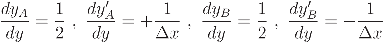
In graphlet 3.1.1: the labels 'A' and 'B' refer both to the midpoints of the respective line elements, and to the two line elements themselves.
For the slope of each line element we use Lagrange notation, indicating the derivative of y with respect to x as y'

To set up for later use we take the derivative with respect to y
With the above preparation in place:
Let CA be the surface area of cone A, CB the surface area of cone B.
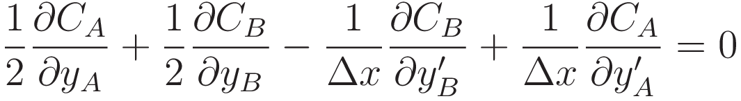
For the pair of adjacent cones of the unit of operation we have the condition: the derivatives with respect to change of the y-coordinate must match, as depicted in graphlets 2.3 and 2.4. The following construction expresses that condition:
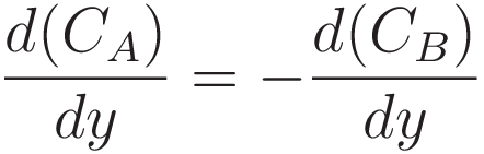
Notice what is not there: (3.1.3) does not evaluate the total area directly. (3.1.3) expresses comparison of the rate of change two adjacent subsections. However, the constraint is that (3.1.3) is to be satisfied over the whole length of the curve concurrently. That is how (3.1.3) relates to the total area.
From (3.1.3) a differential equation is constructed. Solving that differential equation gives the shape of the soap film.
(3.1.3) is stated in terms of elements with a finite size, the cones CA and CB. The final step towards the differential equation will be to take the limit of Δx → 0
Incidentally: while our goal is to find a function that gives the y-coordinate as a function of the x-coordinate, equation (3.1.3) states differentiation with respect to y instead of differentiation with respect to x. That makes (3.1.3) a distinct type of differential equation.
We have to accommodate that the area of the truncated cone involves multiplying the y-coordinate with (a function of) the derivative of the y-coordinate. That means that in order to evaluate (3.1.3) we must expand into partial differentiation.
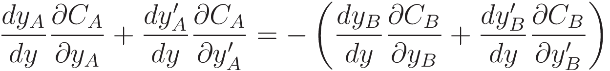
The leading part of each of the four terms of the equation is there because the chain rule has been applied.
First step of developing (3.1.4): substitute the terms of (3.1.2) into it.
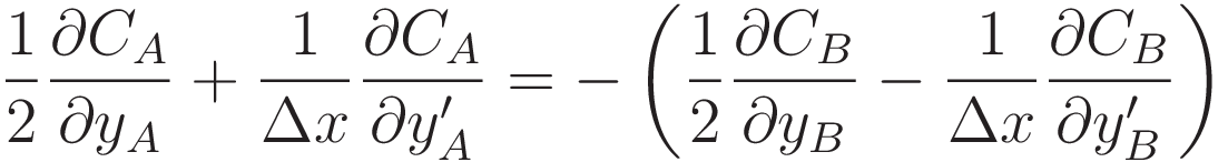
Distribute the minus sign.
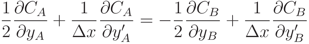
Move the terms on the right hand side to the left and restructure. In (3.1.6) the terms with CA and CB were grouped together, in (3.1.7) the two terms with y are side-by-side, and the two terms with y' are side-by-side.
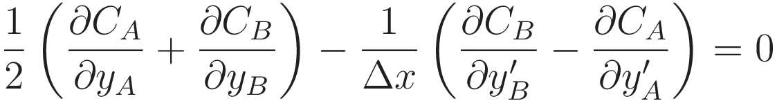
The expression is now at a point where it is ready to take the limit of Δx → 0
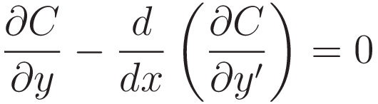
In the limit of Δx → 0:
- the term on the left approaches the partial derivative of C with respect to y.
- The term on the right: between the parenthesis is a difference. It is how much the term (∂C/∂y') changes from the interval x1x2 to the interval x2x3. In the limit of Δx → 0 that is the derivative with respect to x of (∂C/∂y')
Discussion
I encourage you to open a second instance of this page in an adjacent browser window and to scroll to graphlet 2.5. Take the time to understand that (3.1.9) expresses the process that is implemented in the graphlet. In graphlet 2.5 the number of instances of the unit of operation is finite; (3.1.9) is what you arrive at in the limit of infinitesimally small increments.
The form of (3.1.9) is the result of regrouping the derivation (the step from (3.1.6) to (3.1.7)).
3.2 Integration of a test function
This section presents the way of arriving at the Euler-Lagrange equation that in textbooks is most commonly presented: variation is applied to a test function, with evaluation of how the integral responds to that.
Notation:
| y(x) | the function that we want to solve for. |
| ε | multiplication factor |
| yε(x) | test function to execute the variation |
Depiction of the test function yε(x)
Graphlet 3.2.1 demonstrates the way to implement the test function yε(x). A single parameter is used to sweep out variation. Variation of the multiplication factor ε sweeps out the variation of the test function yε(x).
It is sufficient for the test function yε(x) to have the following property:
yε(a) = yε(b) = 0
Noteworthy: the start point and end point used in this derivation do not have to correspond to physical points of the actual problem setting. Working out how to fit the curve to the problem setting comes only later.
The derivation of the Euler-Lagrange equation has the property that at every step the reasoning is independent of the following two properties of the test function:
- which section along the curve the points 'a' and 'b' are located.
- the distance between the points 'a' and 'b'.
Phrased differently: we have the option of thinking of the variation implemented as a single variation, spanning a significant length, but we can also think of the variation as multiple instances, with arbitrarily short span, distributed over the length of the curve. The logic of the derivation is independent of those implementation details.
The setup:
![I[y(x) + \epsilon y_{\epsilon}(x)] = \int_a^b F \big( \ y(x) + \epsilon y_{\epsilon}(x), \ y'(x) + \epsilon y_{\epsilon}^\prime(x) \ \big) dx](../variations_img/20230605_095700_1468x151.png)
Here the integrand of the integration is stated with a capital letter F, to express that it is distinct from the function we are trying to obtain.
To dismiss the integration
The goal now is to arrive at an expression that without ever evaluating the integral will allow us to solve for the curve we are looking for; the goal is to get to a point where we can dismiss the integration.
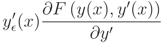
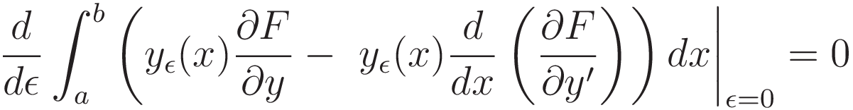
We set up a derivative with respect to the multiplication factor ε. Note that while we do need the ability to take the derivative with respect to ε, we don't need it for a range of values of ε. The derivative with respect to ε at the point where ε is zero is all we need.
![\frac{d}{d\epsilon} I[y(x) + \epsilon y_{\epsilon}(x)] \bigg\rvert_{\epsilon=0} = 0](../variations_img/20230605_101300_647x151.png)
Applying the chain rule:

In order to make progress (3.2.3) must be brought to a form where the test function yε(x) can be dismissed.
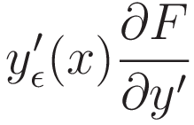
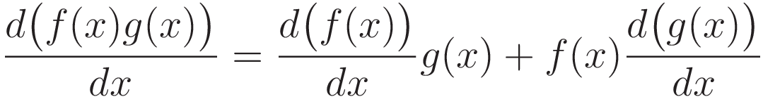
In (3.2.3) the obstacle to progress is the fact that it contains the derivative of yε(x) with respect to x. We will use the product rule of differentiation to transfer that differentiation from the test function yε(x) to the expression F(y(x),y'(x)).
The following term from (3.2.3) is the one that will be transformed:
To save space: from here (3.2.4) will be notated as follows:
The expressions (3.2.6), (3.2.7), (3.2.8), and (3.2.9) cover that transformation process, the transformation process converts (3.2.3) to (3.2.10)
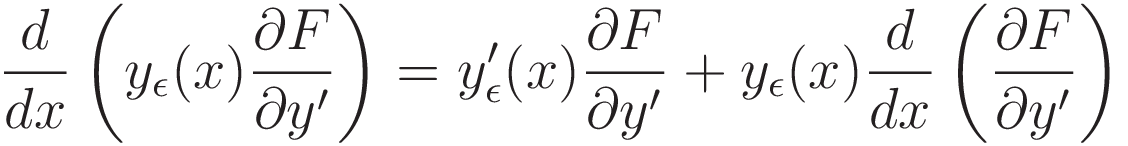
The tool that will be used is the product rule of differentiation:
In (3.2.7) the term we want to transform is the first term on the right hand side of the expression. Everything around that is arranged in such a way that the form of (3.2.7) matches the pattern of (3.2.6).
Set up integration of both sides of (3.2.7), from point a to point b:
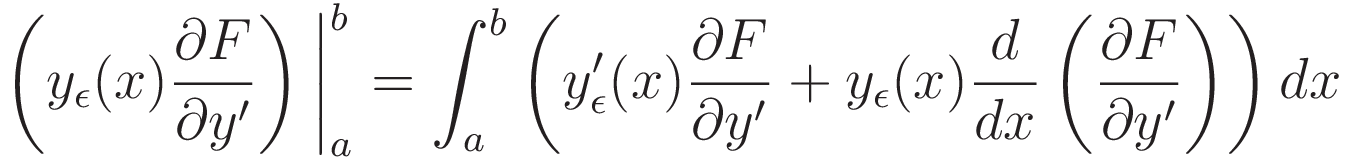
(3.2.8) is the reason why at the start the test function yε(x) was specified to be zero at x=a and x=b.
Given that yε(a) = yε(b) = 0 it follows that the left hand side of (3.2.8) evaluates to zero, hence:
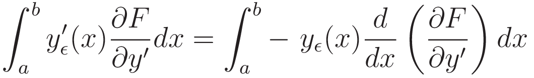
Noteworthy: this transfer of the differentiation is the only point in the derivation where yε(a) = yε(b) = 0 is used. It is not used anywhere else. And again: the logic of this transfer step has no dependence on the positions of a and b. They can be positioned anywhere along the curve, including arbitrarily close together.
The relation (3.2.9) allows us to transform (3.2.3) into the following:
Now that the differentiation has been transferred we can factor out the term yε(x):
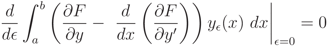
At the start it was announced: we want to get to a point where we can dismiss the test function yε(x), and the integration. With (3.2.11) we have reached that point.
In order to satisfy (3.2.11) we must have:
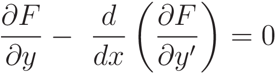
Discussion
The most important feature of the derivation of the Euler-Lagrange equation is this: the integration is dismissed. Dismissing the integration is the whole point of the derivation.
That raises the question: how can it be that while the integration is dismissed we are still able to solve the problem? The explanation: the expression has been shifted to something of equal mathematical power: a differential equation.
A differential equation asserts a global condition in the sense that the solution to the differential equation is a function that satisfies the differential condition concurrently everywhere along the curve.
This was first discussed/demonstrated in graphlet 2.5, the process to find the point of global concurrent equilibrium
The Catenary problem
As announced in the overview, instead of proceeding directly to solve the soap film problem I first move to the Catenary problem.
The catenary problem is first solved with differential calculus, and after that with calculus of variations. The reason for that order will be explained.
4 The catenary
4.1 Introduction
Catenary
In Graphlet 4.1 the length of chain between the cusps is in the catenary shape. I will refer to that specific section - between the cusps - as 'the catenary'. The vertical lines left and right represent chain length hanging down from the respective cusps, providing tensioning force. I will refer to those sections as 'tensioning chain'.
I will refer to the total tension force exerted by the catenary (at the cusp) as the cusp tension. In the diagram the force that the catenary exerts at the cusp is decomposed in two components. The magnitude of the vertical component is equal to the weight of the length of chain that is being suspended in between the cusps. The magnitude of the horizontal component follows from the angle of the chain (at the cusp).
The two piles of chain left and right represent that surplus chain piles up at a set height below the cusp. Only the free hanging length of chain contributes to tensioning, therefore the tension force is for all lengths of the catenary the same. I will refer to this tension as the provided tension.
The cusp tension and the provided tension are acting in opposition to each other; I will refer to the resultant effect as non-equilibrium.
With the checkbox 'Non-equilibrium' checked: the number displayed indicates for the given length of the catenary the state of the opposing forces. As you move the slider left and right: a negative value of the non-equilibrium state means there is not enough provided tension, and when released from that position the catenary will sag. Interestingly, it turns out there are two cross-over points. As you move the slider: the second cross-over point is at slider value 1.44
With the checkbox 'Length' checked: the value that is displayed is the length of chain from cusp to midpoint. The vertical component of the cusp tension is equal to the length of the catenary.
When the catenary is at its equilibrium position: the provided tension is counteracting both the vertical component and the horizontal component of the cusp tension. That is why the provided tension has to be larger than the vertical component of the cusp tension.
Coordinate system of the diagram
The coordinate system is chosen such that the two cusps are located at x=-1 and x=1 respectively. The mass of the chain is set to one unit of mass per unit of length. The provided tension is set up such that at the equilibrium position the horizontal component of the tension in the catenary comes out as 1 unit of force. That is why when the slider is in the 1.00 position the line that represents the horizontal component of the tension force is 1 unit long; it represents 1 unit of force.
4.2 The Catenary in terms of force equilibrium
Graphlet 4.2.1 illustrates why the solution of the catenary problem can be found with a differential equation.
The tension along the catenary
Since the shape is symmetric it is sufficient to evaluate from the midpoint to the cusp.
With:
| TH | The horizontal component of the tension |
| λ | The weight per unit of length |
| L | the length of the chain from the midpoint to the x-coordinate. |
The weight that has to be supported at coordinate x is given by multiplying the length L with the weight per unit of length: λL
In graphlet 4.2.1: move the slider and pay attention to the force component in horizontal direction. Everywhere along the curve that horizontal component has the same magnitude. (The reason that component is a constant: it is perpendicular to the direction of gravity.) For later reference: we can think of this constant as a conserved quantity. In the calculation: as the evaluation traverses the x-coordinate there is a conserved quantity.
Constructing the differential equation
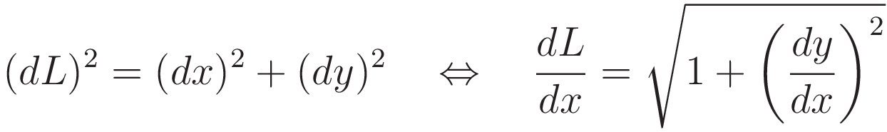
To prepare for later use: from midpoint to cusp the slope of the curve increases; the length of chain per unit of x-coordinate increases accordingly. (4.1) gives an expression for dL/dx.
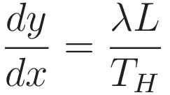
The equilibrium shape has the following property: at every point along the length of the chain the tension force is tangent to the local slope.
At every point, from the mid point to the cusp, the chain above that point is providing the required force to support the weight of the length of chain below that point.
It follows: at every point along the curve: the slope of the curve (the tangent) coincides with the ratio of horizontal tension component and vertical tension component:
On how to proceed from here:
(4.2.2) has a factor L for the length of the chain from the midpoint to the x-coordinate. We need to substitute the factor L with an expression that is purely in terms of the cartesian coordinates x and y. That is why (4.2.1) was prepared.
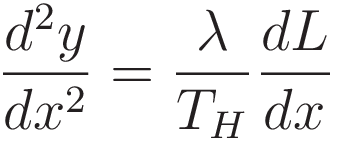
(4.2.1) gives the derivative of L with respect to x, so in order to combine we need to adapt (4.2.2).
At this point we take advantage of the following: the horizontal tension component is a constant. We differentiate both sides of (4.2.2) with respect to x; the factor TH carries over unchanged since it isn't a function of x.
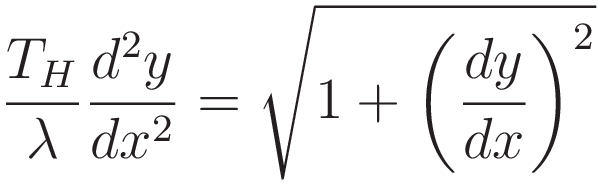
Combining (4.2.3) and (4.2.1) achieves the goal of converting the quantity dL: (4.2.4) is in terms of the cartesian coordinates x and y only:
(Thanks to Daniel Rubin for pointing out the following strategy to solve (4.2.4).
Youtube video: the Catenary )
(4.2.5) is (4.2.4) with the factor TH/λ omitted.
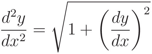
We make the substitution 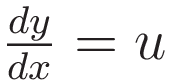 , and we square both sides. Squaring both sides introduces an extraneous solution, so at a later stage we must discard that.
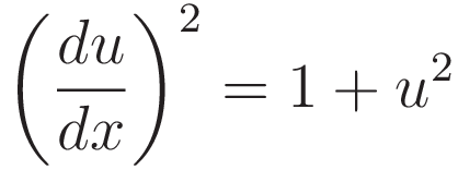
Next we take the derivative with respect to x:
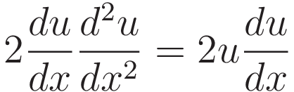
Dividing both sides by 2du/dx:
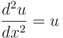
So the solution to the equation is a function with the property that if you differentiate it twice you are back to the original function. That narrows the options down to the following two expressions, which are named 'hyperbolic cosine' and 'hyperbolic sine' respectively:
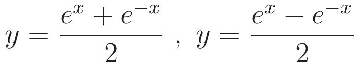
Of these two the first one satisfies (4.2.5)
4.3 The Catenary in terms of minimized potential energy
As long as a hanging chain is still swinging there is interconversion of kinetic energy and potential energy. As the chain swings kinetic energy dissipates to heat. The final state is one where there is no longer opportunity to dissipate energy.
It follows that the hanging chain must have the following property: everywhere along the length any change of the shape will result in a shape that has a higher potential energy than the rest state. The catenary curve is that curve such that among all curves the potential energy is minimal.
We will need an expression for the potential energy. When height difference is small compared to the Earth's radius we can treat the Earth's gravity as a uniform force.
We have that potential energy is defined as the negative of work done; to obtain the work done: integration of force over distance.
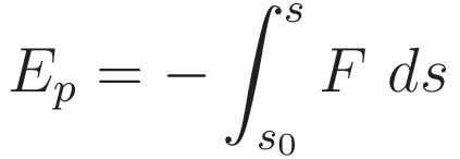
In the case of a uniform force that integration simplifies to multiplication. For gravity the change in potential energy from height h0 to height h:
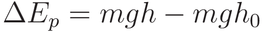
In order to keep the expression simple we set the value of all the constants to 1 unit, and we set h0 to zero. Then the value of the potential energy is equal to the value of height h
In a diagram we will use the y-coordinate for the height h
At this point we are in a position to see what is going to happen.
We have that the Euler-Lagrange equation implements the process that is depicted in the graphlets 2.3, 2.4, and 2.5. The Euler-Lagrange expression is an operator that performs differentiation with respect to the y-coordinate.
(4.3.1) expresses the definition of potential energy: the integral of force with respect to the y-coordinate.
As we know: the operations of differentiation and integration are each other's inverse.
In the case of the catenary: the Euler-Lagrange operator will convert the potential energy to the corresponding force.
Resuming the minimized potential energy approach:
The integral of the potential energy, from midpoint to a cusp located at coordinate x comes out as follows:
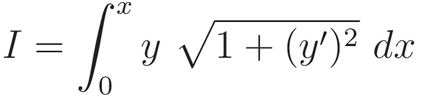
The factor y of the integrand is for the height above zero, and the factor √ (1+(y')²) is for the amount of chain length per unit of distance along the x-axis
As announced earlier, the catenary problem is a sibling of the minimal surface problem; (4.3.3) has the same form as (3.3.2), the integral for the surface area of the soap film.
To solve for the curve of minimal potential energy we use the same strategy as in the case of the differential equation approach: we take advantage of the catenary's property that the horizontal tension component is a constant.
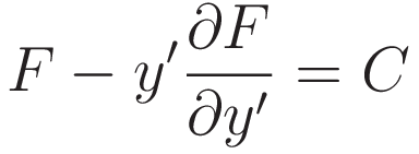
In (4.3.3) the integrand has the terms 'y' and 'dy/dx', but no term with the x-coordinate by itself. That circumstance allows a way to reduce the Euler-Lagrange equation down to a simpler expression. That simpler expression is named 'Beltrami identity'.
Derivation: Appendix I: the Beltrami identity
The Beltrami identity: if 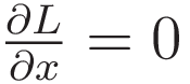 then:
then:
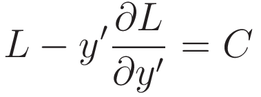
where C is a constant.
Inserting the integrand of (4.3.3) into (4.3.4) gives (4.3.5). The expression looks difficult, but many of the terms drop away against each other.
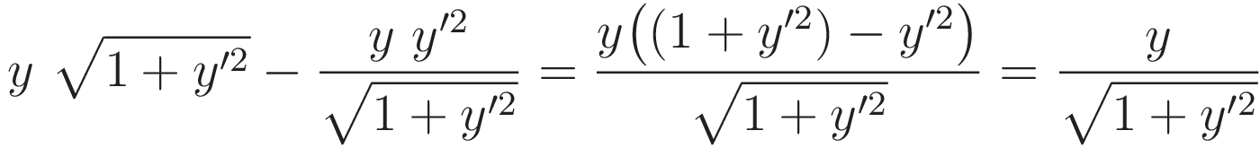
Set equal to a constant C
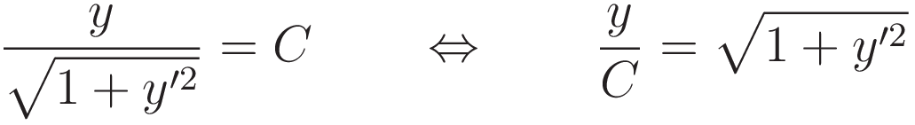
For the time being we set the value of the constant C to '1'.
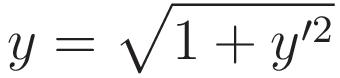
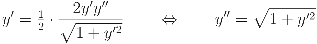
The following is of particularly importance: differentiation with respect to x turns (4.3.7) into (4.2.5)
I encourage you to have two instances of your browser open, putting (4.2.5) and (4.3.8) side-by-side.
We see that the differential approach and the variational approach merge onto the same track. Given the nature of calculus of variations this merger is something that must happen. The reason why is discussed in the next section, section 4.4
4.4 Discussion: relation between force equilibrium approach and energy minimization approach
In order to state the catenary problem as a problem of minimal potential energy: the potential energy (as a function of the height 'h') was obtained from the gravitational force (as a function of the height 'h').
Next that expression is inserted in the Euler-Lagrange equation. The Euler-Lagrange operator specifies differentiation with respect to the y-coordinate. That is: the Euler-Lagrange equation for the catenary does the inverse of how the potential energy was obtained from the force; differentiation versus integration. So we see: the Euler-Lagrange equation for the catenary converts the expression in terms of potential energy back to an expression in terms of force.
The implication:
While it appears as if there are two distinct approaches to solving the catenary problem:
- evaluating force equilibrium,
- minimizing potential energy,
in actual fact the two approaches are one and the same.
The Euler-Lagrange equation performs the type of operation that is visualized in graphlet 2.5; in the limit of the increments along the x-axis approaching zero you get the Euler-Lagrange equation.
Key point:
The way the variational approach solves the catenary problem is an instance of a recurring theme:
The Euler-Lagrange operator converts the potential energy to the corresponding force. The resulting equation is a force equilibrium equation.
5 Classical Mechanics
Main article:
application of Calculus of Variations in Classical mechanics
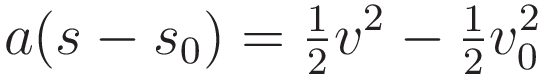
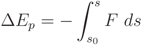
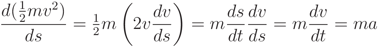
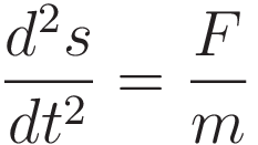
In preparation for later use we will first work out the case of integrating a non-uniform acceleration a from a starting point s0 to an end point s.
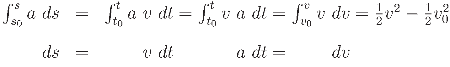
The second row marks the change of differential. For each change of differential the limits change accordingly.
with the intermediate steps omitted:
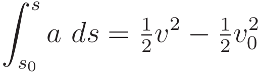
Incidentally: a remarkable property of (5.1) is this: the form of the right hand side is identical to the case of uniform acceleration
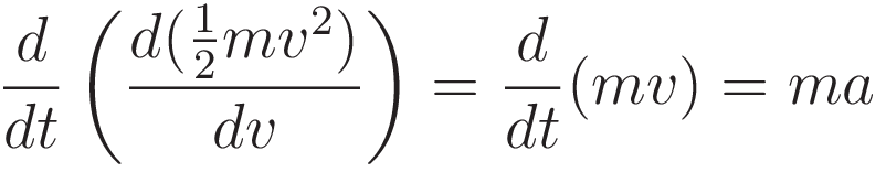
In order to use the Euler-Lagrange in classical mechanics we must construct quantities such that when they are inserted in the Euler-Lagrange equation the Euler-Lagrange equation will recover F=ma
We have that the Euler-Lagrange operator performs differentiation with respect to the position coordinate. Therefore we start with F=ma and we integrate both sides with respect to the position coordinate.
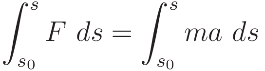
We use (5.1) to develop the right hand side:
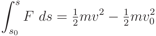
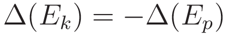
(5.4) is the work-energy theorem. The left hand side of (5.4) is work done, and the left hand side is kinetic energy.
Potential energy is defined as the negative of work done.
About the concept of kinetic energy: there was a precursor concept, which was named vis viva, 'the living force', defined as mv². Around the mid 1800's the physics community shifted to a kinetic energy defined as ½mv².
Clearly the shift to ½mv² was bound to happen: defining kinetic energy in accordance with the work-energy theorem makes everything fit together.
A prominent example of this everything-fits-together: with potential energy and kinetic energy defined in accordance with the work-energy theorem we have: in interconversion of potential energy and kinetic energy the amount of change of energy matches:
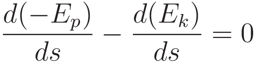
Since potential energy and kinetic energy are obtained by integration with respect to the position coordinate: differentiating with respect to the position coordinate will recover F=ma:
(5.7) can be restated in a form of that coincides with the form of the Euler-Lagrange equation.
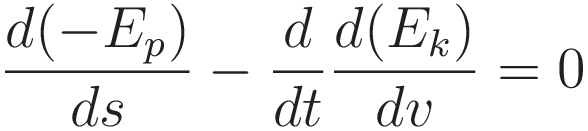
(5.9) and (5.10) demonstrate the equivalence of (5.7) and (5.8): (5.9) and (5.10) both evaluate to ma.
Discussion
The Euler-Lagrange expression is an operator that performs differentiation with respect to the y-coordinate.
In the context of the catenary problem it is customary to treat the horizontal position coordinate as the x-coordinate, making the y-coordinate the height coordinate h. Thus in the case of the catenary problem the Euler-Lagrange equation performs differentiation with respect to the height coordinate, converting the potential energy to force.
In the context of classical mechanics the goal is to obtain the position coordinate of some object as a function of the time-coordinate. Thus in the case of classical mechanics the Euler-Lagrange equation performs differentiation with respect to the position coordinate, converting potential energy to force, and the ½v² part of the kinetic energy to acceleration.
In the case of Classical Mechanics: to apply the Euler-Lagrange equation is to find the point in variation space such that everywhere along the trajectory the rate of change of kinetic energy matches the rate of change of potential energy.
In the case where the potential energy is expressed in terms of some form of generalized coordinates, see Appendix II: generalized force
Appendix I: the Beltrami identity
The relation between the Euler-Lagrange equation and the Beltrami identity is: the Beltrami identity is the Euler-Lagrange equation with a differentiation with respect to x backed out.
Preparation for later use:
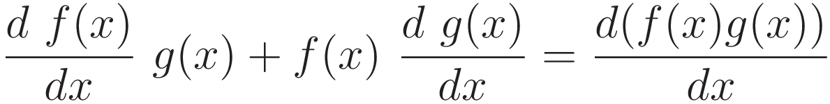
The product rule for differentiation:
In the derivation of the Beltrami identity the product rule will be used in reverse: it will be used to collapse two terms into one.
In the case of the soap film minimal surface problem and the catenary problem: there is no direct dependence on the x-coordinate. The integrand has the terms 'y' and 'dy/dx', but no term with the x-coordinate by itself
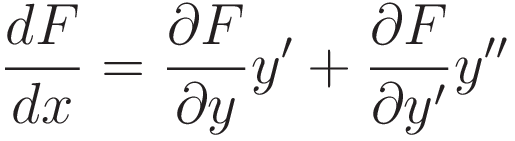
the general expression for the derivative of F with respect to x has three terms: one for x, one for y, and one for y':
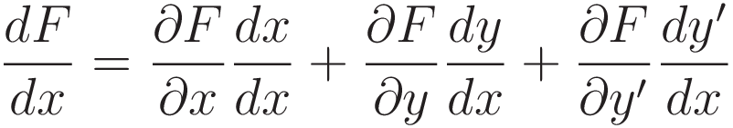
The objective is to derive an expression for a subset of the general set, the subset such that the partial derivative with respect to x is zero. So: that partial derivative is dropped.
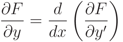
In order to go from The Euler-Lagrange equation to the Beltrami identity we need to accomplish the following three objectives:
- Combine (I.4) and the Euler-Lagrange equation
- Collapse the two terms on the right hand side of of (I.4) into one term
- That one term must be one of differentiation with respect to x
We use the following form of the Euler-Lagrange equation to substitute the term ∂F/∂y that is on the right hand side of (I.5):
Some rearranging:
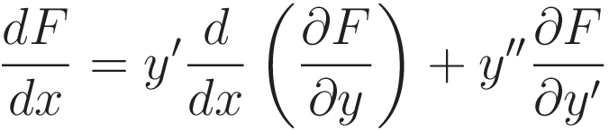
The substitution has in fact accomplished all three of the objectives:
At this point the product rule is applied in reverse: the two terms on the right hand side of (I.6) have the same pattern as the left hand side of (I.2) so they can be folded into a single term.
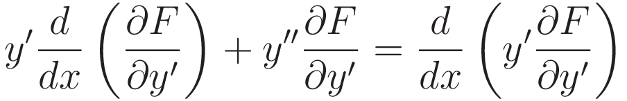
(I.8) is (I.6), with the right hand side substituted according to (I.7).
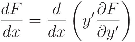
Since differentiation is a linear operation we can factor it out:
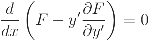
The fact that a differentiation with respect to x can be factored out is not a coincidence, of course. (I.5) expresses the property that the derivative of F with respect to x is zero. That is why we ended u being able to back out a differentiation with respect to x
In order to satisfy (I.9) the expression inside the parentheses must be a constant. That statement is the Beltrami identity.
Return to where the Beltrami identity is used
Appendix II: generalized force
When the potential energy is expressed in terms of some form of generalized coordinate(s) the result of differentiation with respect to the position coordinate will be an expression in terms of a generalized force.
The concept of generalized force is to be understood as follows:
Example:
Let's say that we are modeling the oscillation of the balance wheel of a watch, using:
- polar coordinates
- rotational kinetic energy
- potential energy of a spiral shaped spring.
Then the Euler-Lagrange equation does the following conversions:
- potential energy to torque
- the ½ω² part of rotational kinetic energy to angular acceleration.
Torque is an example of a generalized force. It is of course the most widely known example of it.
At this point we consider the form of F=ma.
F=ma expresses a relation between the following three types of entity:
- tendency to cause change of state (force)
- coefficient of opposition to change of state (inertia)
- second time derivative of the position coordinate
The ratio of the force and the opposition to change gives the resulting acceleration, the second time derivative of position.
In the case of a balance wheel it is convenient to use polar coordinates, and then the dynamic entities come out as torque, moment of inertia, and angular acceleration.
The corresponding equation that gives the angular acceleration as a function of the ratio of torque and moment of inertia:
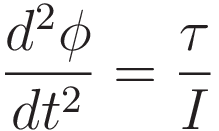
| τ | torque |
| I | moment of inertia |
| φ | angle |
This pattern generalizes to all forms of generalized coordinates.
As we know: torque does not have the dimensions of force. For self-consistency: for a given choice of coordinate the corresponding generalized force must be such that the product of generalized force and its corresponding generalized coordinate has the dimensions of work.
Reference:
Richard Fitzpatrick, Classical Mechanics course:
Generalized forces
It is to be expected that the form of the fundamental equation is independent of the choice between cartesian coordinates and some form of generalized coordinates. Indeed: in classical mechanics the fundamental equation has the same form independent of the choice of coordinate system. The three dynamics entities are:
- agent of change (force, torque, etc.)
- opposition to change (inertia, moment of inertia, etc.)
- second time derivative of position coordinate
The expressions (II.1) and (II.2) have been set up to illustrate that the form of the fundamental equation is independent of the choice between cartesian and (some form of) generalized coordinate(s).

This work is licensed under a Creative Commons Attribution-ShareAlike 3.0 Unported License.
Last time this page was modified: April 28 2025