Remark:
In this article I'm assuming that the reader is comfortable with the physics that was discussed in the previous articles of the Coriolis effect series. In particular, I'm assuming the reader is at ease with the information in the articles about Rotational-vibrational coupling and Oceanography: inertial oscillations

The Foucault pendulum

Picture 1. Animation
A Foucault pendulum located at 30 degrees latitude takes two sidereal days to complete a precession cycle.

Stereographic animation
(Switches to other page.)

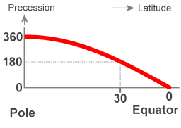
Picture 2. Diagram
The precession with respect to the Earth's surface in degrees per sidereal day.

A Foucault pendulum located at the latitude of Paris takes about 32 hours to complete a precession cycle. This means that after one sidereal day, when the Earth has returned to its orientation of one day before, the pendulum has precessed three quarters of a cycle. If it has started in north-south direction, it is swinging east-west when the Earth has returned to the orientation of one day before.

Animation 1 represents another example, the case of a Foucault pendulum located at 30 degrees latitude. One can recognize that the plane of swing takes two sidereal days to precess clockwise with respect to the surface it is suspended above. At the equator the pendulum keeps swinging in the same direction relative to the surface it is suspended above. Diagram 2 depicts that from the poles to the equator there is a smooth transition.

The challenge is to explain the behavior of a Foucault pendulum that is not located on either the poles or the equator. Many discussions of the Foucault pendulum merely rephrase the observation. For instance, Hart, Miller and Mills point out that "the angular velocity of the plane of the pendulum is simply the projection of the Earth's angular velocity onto a line joining the center of the Earth and the point of suspension of the pendulum".¹ That's an empty statement; it just restates the already known.

A satisfactory explanation of the motion pattern of the latitudinal Foucault pendulum has been given by meteorologists². The fact that meteorologists have made a crucial contribution is not as surprising as it seems. Air mass, the object of study in meteorology, is pretty much prevented from moving in vertical direction, but there is hardly any restraint to motion parallel to the local Earth surface. Likewise, the pendulum bob has no freedom in vertical direction, but it is unconstrained in the directions parallel to the Earth's surface. Whenever air mass has a velocity relative to the Earth there is an effect that arises from the overall Earth rotation. Likewise, the fact that the swinging pendulum is circumnavigating the Earth's axis affects the motion of the pendulum.

I will call a Foucault pendulum located on one of the poles a polar Foucault pendulum and a Foucault pendulum located somewhere on the equator an equatorial Foucault pendulum. A Foucault pendulum located at any latitude between the poles and the equator I will call a latitudinal Foucault pendulum.

The motion pattern of the Foucault pendulum involves two oscillations, at different scales of magnitude. At the small scale there is the swing of the pendulum, which I will refer to as 'the vibration'. At the large scale there is the overall rotation of the Earth around its axis. The vibration participates in the overall rotation and is affected by it. Due to the large difference in period of oscillation the effect is very small during each separate swing. It appears to be negligable, but it's actually significant because the effect is cumulative. My purpose is to show why the effect is cumulative.

Table of contents

· The Wheatstone-Foucault device
· The Wheatstone pendulum
· Physics principles
    · Wheatstone pendulum forces
    · Foucault pendulum forces
    · Decomposition in vector components
    · Exchange of angular momentum
    · The sine of the latitude
    · Applicability
· Mathematical derivations
    · The two forces in the equation of motion
    · The centrifugal term and the Coriolis term
    · The full equation of motion
    · What the equation describes
· Overview: the centripetal force doing work
· Historical note

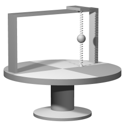
The Wheatstone-Foucault device

Picture 3. Image
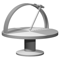
Wheatstone's design that displays the same effect as the Foucault pendulum.

In 1851 a paper by Charles Wheatstone was read to the Royal Society in which Wheatstone described the device that is shown in Image 3. A transcript of the paper by Wheatstone is available at wikisource: Note relating to M. Foucault's new mechanical proof of the Rotation of the Earth"

The helical spring acts as a heavy string; when plucked, it vibrates. The circular platform can rotate around a vertical axis. I will refer to this axis as the central axis.

The Wheatstone pendulum

Picture 4. Image
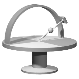
Version of Wheatstone's device that underlines the similarity with the Foucault pendulum.

Picture 5. Image
A Wheatstone pendulum setup with the attachment points aligned with the central axis of rotation.

I will discuss the physics of the Foucault pendulum by drawing parallels with Wheatstone's device. The features that the Foucault pendulum and the Wheatstone-Foucault device have in common are the features that matter for understanding the physics taking place.

To underline the similarity with the Foucault pendulum, I will discuss a slightly different version of the Wheatstone-Foucault device. I refer to the device depicted in image 4 as "the Wheatstone pendulum". The small sphere corresponds to the bob of the Foucault pendulum, the force exerted by the inside spring corresponds to the gravitational force that is being exerted on the bob, and the force exerted by the outside spring corresponds to the force that the pendulum wire exerts on the bob.

The University at Buffalo, State University of New York physics department has a permanent exhibition that includes a tabletop model. The tabletop model uses an elastic pendulum to emulate a Foucault pendulum at 43° degrees latitude, the latitude of Buffalo, New York.

Other examples of such a tabletop mechanical model demonstrating the Foucault effect:

Working Model of a Foucault Pendulum at Intermediate Latitudes
Francis W. Sears
Am. J. Phys. 37, 1126 (1969)
A new model of the Foucault pendulum
Klaus Weltner
Am. J. Phys. 47, 365 (1979)

Finally, Image 5 depicts yet another version of the device that I will use later to focus on a particular factor that is involved in the motion pattern of the Foucault pendulum. The suspension points are aligned with the central axis, but the bob is located at some distance from the central axis.

Physics principles

The assumptions for the purpose of simplifying the analysis.

All of the mass of the bob is taken as concentrated in the midpoint of the bob
The springs are taken as massless.
The range of motion of the bob with respect to the rest state is taken to be within the limits of the small angle approximation.
Only the forces exerted by the springs are considered.

Wheatstone pendulum forces

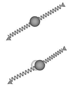
Picture 6. Image
Top: rest state.
Bottom: outward displacement of pendulum bob when platform is rotating.

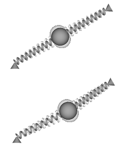
Picture 7. Image
Top: vibration pattern while platform is not rotating.
Bottom: vibration with rotating platform.

Images 6 and 7 show a detail of the Wheatstone pendulum, in different states of motion.

Image 6:
The top side of the image shows the shape of the springs when the Wheatstone pendulum is not in motion. Both springs are equally stretched, and they are aligned. The bottom side of the image illustrates the outward displacement of the pendulum bob when the platform is rotating. The inner spring is more extended than in the rest state, the outside spring is less extended than in the rest state, and thus the springs provide the required centripetal force to make the pendulum bob circumnavigate the central axis of rotation.

Image 7:
The top side of the image shows the shape of the springs when the Wheatstone pendulum is vibrating, but not rotating around the central axis. Both springs are equally stretched, and at the equilibrium point they are aligned. The bottom side of the image shows that when the pendulum bob is vibrating while the platform is rotating the midpoint of the vibration is the outward displaced point of the pendulum bob.

Picture 8. Diagram
The forces in the case of a plumb line.
Blue arrow: the actual gravitational force, pointing towards the center of attraction.
Red arrow: the force exerted by the suspending wire.
Green arrow: the resultant force.

Foucault pendulum forces

Image 8 depicts the forces in the case of a plumb line. It's necessary to distinguish between true gravity and effective gravity. In the diagram the blue arrow represents true gravity, it is directed toward the center of gravitational attraction. On a non-rotating celestial body true gravity and effective gravity coincide, but in the case of a rotating celestial body (due to the rotation deformed to a corresponding oblate spheroid) some of the gravity is spent in providing required centripetal force. (For a quantitative discussion, see the 'differences in gravitational acceleration' section in the Equatorial bulge article.) Due to the rotation the plumb line swings wide. The plumb line's equilibrium point is the point where the angle between true gravity and the tension in the wire provides the required centripetal force.

Of course, since inertial mass is equal to gravitational mass a local gravimetric measurement cannot distinguish between effective gravity and true gravity. Nevertheless, for understanding the dynamics of the situation it is necessary to remain aware that at all times a centripetal force is required to sustain circumnavigating motion.

At 45 degrees latitude the required centripetal force, resolved in the direction parallel to the local surface, is 0.017 newton for every kilogram of mass. In the case of the 28 kilogram bob of the Foucault pendulum in the Pantheon in Paris that is about 0.5 newton of force. If you have a small weighing scale among your kitchen utensils then you can press down on it and feel how much force corresponds to a weight of 50 grams. (2.2 pounds corresponds to 1 kilogram.) Or you can calculate how much centripetal force you are subject to yourself, and then use the scale to feel how much force that is. If you weigh 75 to 80 kilogram you are looking at about 150 grams of force. The angle between true gravity and the direction of the plumb line provides that force.

The angle between true gravity and a plumb line at 45 degrees latitude is about 0.1 of a degree. For the Foucault pendulum in the Pantheon, with a length of 67 meters, the corresponding horizontal displacement is 0.11 meter. (Interestingly, for the pendulum in the Pantheon Foucault has documented that on occasion there was opportunity for uninterrupted runs of six to seven hours. As far as he could tell the precession rate remained the same. William Tobin writes in his biography of Foucault that according to calculations after 7 hours friction will have reduced the amplitude of the swing to about 0.1 meter.)

Decomposition of the force

Picture 9. Graphlet

Picture 9 is an interactive diagram. The red dot is draggable. The two horizontal lines are sliders.

The blue dot represents the central rotation axis. The green dot is circumnavigating the blue dot. The green vector represents the actually exerted force. For simplicity this force is treated as a perfect harmonic force; a force that is at every point proportional to the distance to the midpoint. The blue vector represents required centripetal force.

The brown vector is the green vector minus the blue vector. The grey dot represents the displaced midpoint of the vibration. The brown vector can be thought of as a restoring force towards the displaced midpoint of the vibration.

The sliders adjust the size of the required centripetal force and the actually exerted force respectively.

Purpose of the decomposition

The derivation of the equation of motion further down in this article uses the components, not the actually exerted force. The advantage: in the equation of motion for the rotating coordinate system the required centripetal force term and the centrifugal term drop away against each other.

Exchange of angular momentum

Picture 10. Image
A Wheatstone pendulum setup with the attachment points aligned with the central axis of rotation.

Picture 11. Animation
Motion of the bob of the device depicted in Image 9.

Picture 12. Animation
Schematic representation of the motion of the bob as seen from a co-rotating point of view.

I will first discuss the motion pattern of the device depicted in image 10.

Let the platform be rotating counterclockwise. To underline the comparison with the Foucault pendulum I will call the the bob's motion in a direction tangent to the rotation 'east-west motion'.

Motion towards and away from the central axis

At every point in time, the bob has a particular angular momentum with respect to the central axis of rotation. When the bob is pulled closer to the central axis of rotation the centripetal force is doing mechanical work. As a consequence of the centripetal force doing work the angular velocity of the bob increases. (Compare a spinning ice-skater who pulls her arms closer to her body to make herself spin faster.) When the pendulum bob is moving away from the central axis the centripetal force is doing negative work, and the bob's angular velocity decreases. The animation illustrates that the effects during the halfswing towards the central axis and halfswing away from the central axis do not cancel each other; the combined effect is cumulative.

Velocity relative to co-rotating motion

The amount of centripetal force that is exerted upon the pendulum bob is "tuned" to the state of co-rotating with the system as a whole. I will refer to the velocity that corresponds to co-rotating with the system as a whole as 'equilibrium velocity'. During a swing of the pendulum bob in eastward direction the bob is circumnavigating the central axis faster than the equilibrium velocity, hence during an eastward swing the bob will swing wide. During a swing of the pendulum bob in westward direction the bob is circumnavigating the central axis slower than the equilibrium velocity, hence during a westward swing there is a surplus of centripetal force, which will pull the bob closer to the central axis. The animation illustrates that the effects during the halfswing from east-to-west and the halfswing from west-to-east do not cancel each other; the combined effect is cumulative.

Java simulation

To further illustrate the symmetries that underly the motion of animation 11 I have created the following 2D Java simulation: Circumnavigating pendulum

Transfer

Swinging towards and away from the central axis is a vibration in radial direction. Swing in tangential direction superimposed on the circumnavigating motion is a vibration in tangential direction. The pendulum bob and the pendulum support are exchanging angular momentum all the time.

Of course, in the case of a Foucault pendulum the entire Earth is effectively the pendulum support. Obviously since the Earth is so much heavier than the pendulum bob the Earth's change of angular momentum is utterly negligable. But as a matter of principle change of (angular) momentum is always in the course of an exchange of (angular) momentum.

Animation 11 shows a remarkable symmetry: the direction of the bob's oscillation with respect to inertial space remains the same, just as in the case of a polar Foucault pendulum!

In the case of a polar Foucault pendulum the fact that the direction of the plane of swing remains the same is due to straightforward conservation of momentum. In the case depicted in image 10 and animation 11 there is a precession relative to the rotating system that precisely cancels the system's rotation. In the section in which I discuss the mathematical treatment I show how that occurs.

The sine of the latitude

Picture 13. Animation
Motion of the bob of the Wheatstone pendulum as seen from straight above the platform. Positioning of the springs (the springs are not shown) corresponds to 30 degrees latitude.

Animation 13 shows the case of the Wheatstone pendulum when it is set to model a Foucault pendulum at 30 degrees latitude. At 30 degrees latitude a full precession cycle takes two days. Compared to the case represented in animation 10 the precession relative to the co-rotating system is slower.

The closer to the equator a Foucaut pendulum is located, the slower its precession relative to the ground it is suspended above. At the equator the plane of swing is completely co-rotating with the rotation of the overall system.

Picture 14. Image
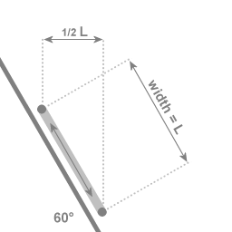
In the case of an angle of 60 degrees with the central axis of rotation: If the two extremal points of the swing are a distance of L apart, then the motion towards and away from the central axis covers a distance of 1/2 L

Image 14 illustrates why the precession is slower at lower latitudes.

The amount of precession (relative to the co-rotating system) is determined by the exchange of angular momentum. At 30 degrees latitude: when the swing from one extremal point to the opposite extremal point covers a distance of L, then the motion towards (or away from) the central axis is over a distance of 1/2 L. So in the case of a setup at 30 degrees latitude the force is half as effective, and the precession is half the rate of a Foucault setup near the poles.

Java applets

I have created a 3D simulation that models the Foucault pendulum

Applicability

The ratio of vibrations to rotations
In actual Foucault setups the ratio of vibrations to rotations is in the order of thousands to one. In the examples given in this article the ratio of vibrations to rotations is in the order of ten or twenty to one. Interestingly, this difference is inconsequential. In both ranges the physics principles are the same; the considerations that are presented are valid for all vibration-to-rotation ratio's.
However, below a ratio of around 10 to 1 and approaching 1 on 1 the motion associated with the rotation and the motion associated with the vibration blur into each other so much that there is no meaningful Foucault effect to be observed.

The amplitude of the vibration
Images 6 and 7 depict a case where the amplitude of the vibration is slightly smaller than the outward displacement of the bob; in the usual setup the amplitude of the vibration is larger than the displacement, much larger. Does this matter? It does not matter in the following sense: one of the properties of the Foucault pendulum is that its precession does not depend on the amplitude of the swing; when the amplitude of a Foucault pendulum decays the rate of precession remains the same. The Java simulations Foucault pendulum and Foucault rod illustrate the property that the rate of precession is independent from the vibration amplitude.

Mathematical derivations

Picture 15. Image
A Wheatstone pendulum setup with the attachment points aligned with the central axis of rotation.

I will start with a derivation for the Wheatstone pendulum setup that is depicted in image 15. That setup is effectively a 2-dimensional case; all forces that are involved act parallel to the plane of the equator; all motion is in a plane that is parallel to the equator. At the very end of the mathematical discussion I will add the modification that generalizes the result to cases where the suspension points are not aligned with the central axis of rotation.

The equation of motion

As discussed in the section Decomposition in vector components the mathematics of the equation of motion is simplified by representing the force exerted upon the pendulum bob as a combination of two forces:

· Centripetal force that sustains the rotation
· Restoring force that sustains the vibration

Both can be treated as a harmonic force.

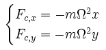
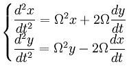
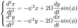
The centripetal force that sustains rotation with constant angular velocity Ω, for a coordinate system with the zero point at the central axis, is given by:

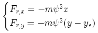
$\begin{cases} F_{c,x} = - m \Omega^2 x \\ F_{c,y} = - m \Omega^2 y \end{cases}$

The restoring force acts towards the equilibrium point (plumb line direction) of the pendulum. The coordinate system can be chosen in such a way that the central axis and the equilibrium point are both on the y-axis. Let the y-coordinate of the equilibrium point be called y_e. Let the frequency of the pendulum swing be called ψ.

$\begin{cases} F_{r,x} = - m \psi^2 x \\ F_{r,y} = - m \psi^2 (y - y_e) \end{cases}$

The centrifugal term and the Coriolis term

I assume that the reader is at ease with the centrifugal term and the Coriolis term. The necessary information is present in the articles Rotational-vibrational coupling and Oceanography: inertial oscillations and in the following interactive animation Coriolis effect. In the rotational-vibrational coupling article I present a derivation of the Coriolis term (the centrifugal term is trivial), and in the inertial oscillation article I show how things work out for terrestrial effects.

To help recognize the notation: in the following system of equations (which is for motion relative to a coordinate system that rotates with angular velocity Ω) the term that is proportional to x and y is the centrifugal term. The Coriolis term is proportional to dx/dt and dy/dt respectively.

The acceleration that is associated with the Coriolis effect is perpendicular to the velocity. If you have a vector dx/dy, then the vector perpendicular to that is -dy/dx; it's the negative, and inverted. In the system of motion equations (for x-direction and y-direction) you see that the factor 2Ωdy/dt is in the equation for acceleration in the x-direction, and vice versa.

$\begin{cases} \dfrac{d^2x}{dt^2} = \Omega^2 x + 2 \Omega \dfrac{dy}{dt} \\ \dfrac{d^2y}{dt^2} = \Omega^2 y - 2 \Omega \dfrac{dx}{dt} \end{cases}$

The full equation

No factor m
Let me explain first why I have omitted the factor 'm' for the mass in the equation of motion below. The restoring force arises from elasticity. If the bob is replaced with a heavier bob then the elastic material stretches some more before settling into an equilibrium state. The required force is proportional to m, and the setup simply self-adjusts to provide the required force.

The full equation of motion for motion with respect to a rotating coordinate system has four factors: the two components of the force plus the centrifugal term and the Coriolis term.

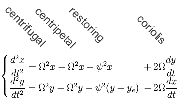
$\begin{cases} \dfrac{d^2x}{dt^2} = \Omega^2 x - \Omega^2 x - \psi^2 x & \!\!\! + \, 2 \Omega \dfrac{dy}{dt}\\ \dfrac{d^2y}{dt^2} = \Omega^2 y - \Omega^2 y - \psi^2 (y - y_e) & \!\!\! - \, 2 \Omega \dfrac{dx}{dt} \end{cases}$

It's assured that 'centrifugal' and 'centripetal' drop away against each other because the system is self-adjusting: if the angular velocity of the system would increase then the springs deform a little more until the point is reached where the springs once more provide the required amount of centripetal force.

Letting the centrifugal term and the expression for the centripetal force drop away against each other:

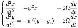
$\begin{cases} \dfrac{d^2x}{dt^2} = - \psi^2 x & \!\!\! + \, 2 \Omega \dfrac{dy}{dt} \\ \dfrac{d^2y}{dt^2} = - \psi^2 (y - y_e) & \!\!\! - \, 2 \Omega \dfrac{dx}{dt} \end{cases}$

This equation of motion describes the effects of the centripetal force on the motion pattern.

The above expression can be simplified further by shifting the zero point of the coordinate system. The Coriolis term only contains velocity with respect to the rotating system, so it is independent of where the zero point of the coordinate system is positioned. In the following equations x and y are not the distance to the central axis but the distance to the center point of the vibration.

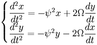
$\begin{cases} \dfrac{d^2x}{dt^2} = - \psi^2 x + 2 \Omega \dfrac{dy}{dt} \\ \dfrac{d^2y}{dt^2} = - \psi^2 y - 2 \Omega \dfrac{dx}{dt} \end{cases}$

As a reminder: the above equations apply for only a single case, the case when the suspension of the pendulum is aligned with the central axis of rotation, as depicted in image 15.

This system of equations is the same as the equations of motion for two coupled oscillators. Here the oscillations are vibration in x-direction and vibration in y-direction. The Coriolis term describes that acceleration in x-direction is proportional to velocity in y-direction, and that acceleration in y-direction is proportional to velocity in x-direction. In other words: the Coriolis term describes the transfer of the vibration direction.

Weakened coupling

Picture 16. Image
In the case of an angle of 60 degrees with the central axis of rotation: If the two extremal points of the swing are a distance of L apart, then the motion towards and away from the central axis covers a distance of 1/2 L

When the attachment points are not aligned with the central axis of rotation the coupling between the rotation and the vibration is weakened. Less motion towards and away from the central axis of rotation means the centripetal force will be doing less work.

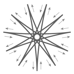
$\begin{cases} \dfrac{d^2x}{dt^2} = - \omega^2 x + 2 \Omega \dfrac{dy}{dt} sin(\phi) \\ \dfrac{d^2y}{dt^2} = - \omega^2 y - 2 \Omega \dfrac{dx}{dt} sin(\phi) \end{cases}$

Picture 17. Image
The shape of the pendulum bob's trajectory.

Obtaining an analytic solution to that equation of motion is in the second Foucault pendulum article

Image 17 has been created by plotting the analytic solution to the above equation of motion. It represents the case where the ratio of ψ to Ω is 11 to 1 (Usually the ratio of ψ to Ω is in the order of thousands to one). The image depicts the case of releasing the bob in such a way that on release it has no velocity with respect to the rotating system.

What the equations describe

Remarkably, the equations describe that the shape of the trajectory of the Foucault pendulum is exactly the same on all latitudes, the latitude of deployment affects only the rate of precession. That means that just from the shape of the trajectory you will not be able to observe the magnitude of the Earth's rotation rate. For instance, if you observe that it takes 32 hours for the pendulum to complete a precession cycle then maybe the Earth takes 32 hours to rotate, or maybe you are on a latitude where the precession takes 32 hours, with the Earth rotating at some unknown faster rate. So if you limit yourself rigidly to using data from the pendulum motion only you cannot observe the Earths rotation rate.

The similarity of the shape on every latitude is quite surprising, for in the case of a polar pendulum and in the case of a latitudinal pendulum the mechanism that is involved is entirely different.
In the case of a polar pendulum the only physics taking place is the swing of the pendulum, the Earth merely rotates underneath the pendulum, without affecting it; the "precession" of a polar pendulum is apparent precession. On the other hand, in the case of a latitudinal pendulum the pendulum setup as a whole is circumnavigating the Earth's axis and consequently the vibration is affected: there is a coupling of latitudinal and longitudinal vibration. When the coupling is 100% as in the setup depicted in animation 10 the vibration retains the same orientation with respect to inertial space. When the coupling is less then 100%, as in the case of a Foucault setup somewhere between the poles and the equator there is an actual precession of the pendulum swing.

Overview: the influence of the centripetal force.

The reason that the centripetal force is crucial is the fact that the direction of the centripetal force is not constant.

For contrast: compare with the case of a displacing force that is constant in direction. Take for instance the following setup: a pendulum suspended in a train carriage that accelerates uniformly in a straight line. That uniform acceleration can be incorporated as a tilt of the vertical (just like a plumb line in a uniformly accelerating train carriage will be tilted accordingly); it will not affect the direction of the pendulum swing.

Cumulative

In the case of a Foucault pendulum the centripetal force does affect the direction of the plane of swing. While the centripetal force's change of direction during each separate swing is minute, it is nonetheless the determining factor because the effect is cumulative.

Historical note.

Gustave Gaspard Coriolis undertook theoretical examination of the efficiency of waterwheels. In the opening paragraph of his article, Coriolis mentions that Bernouilli had analysed the case of what force acts upon an object that can slide freely inside a horizontal tube that is rotating. Coriolis had then taken it upon himself to work out the most general formulas, formulas for handling any motion. These formulas would allow Coriolis to calculate for any shape of waterconduit the amount of work that could be extracted. In the course of deriving formulas, one of the terms that arose was what today is referred to as 'the Coriolis term'.

Coriolis' investigations dealt with mechanical work, his investigations dealt with energy conversion. And in the case of a latitudinal Foucault pendulum the actual precession is due to work being done by the centripetal force.

Next article:
Foucault pendulum: Elaboration

The main sources of information for this article:

Persson, Anders, 1998 How do we Understand the Coriolis Force? Bulletin of the American Meteorological Society 79, 1373-1385.
Persson, Anders The Coriolis effect - a conflict between common sense and mathematics PDF-file. 17 pages. A general discussion by Anders Persson of various aspects of the Coriolis effect, including Foucault's Pendulum and Taylor columns. (PDF-file, 800 KB)
Phillips, N. A., What Makes the Foucault Pendulum Move among the Stars? Science and Education, Volume 13, Number 7, November 2004, pp. 653-661(9)
(Previously published in French: Ce qui fait tourner le pendule de Foucault par rapport aux étoiles La Meteorologie no. 34 august 2001

William Tobin, The life and science of Léon Foucault Biography, published in 2003.

Notes:

note 1
John B. Hart, Raymond Miller, Robert L. Mills, A simple geometric model for visualizing the motion of a Foucault pendulum American Journal of physics 55(1), January 1987

note 2
Authors that I am aware of who discuss the mechanism of the Foucault pendulum's precession.
- Ferrel, W. 1858. The influence of the Earth's rotation upon the relative motion of bodies near its surface. Astron. J., Vol V. No. 109, 97-100. (PDF file, 548 KB, scans of article pages )
- Phillips, N. A., What Makes the Foucault Pendulum Move among the Stars? Science and Education, Volume 13, Number 7, November 2004, pp. 653-661(9)

This work is licensed under a Creative Commons Attribution-ShareAlike 3.0 Unported License.

Last time this page was modified: December 29 2023