This article is under construction.
- Completed: demonstration of using differential calculus to find the equation of the catenary curve.
- Completed: demonstration that identifying the point of minimum potential energy is identical to identifying force equilibrium.
- Still to do: numerical analysis implementation of finding the shape of the catenary curve, using the same implementation structure as applied in diagrams 3.1, 3.2 and 3.3 presented in the article with discussion of Hamilton's stationary action.

This article is part of a set of three; the common factor is Calculus of Variations. In classical physics Calculus of Variations is applied in three areas: Optics, Statics, and Dynamics. Each article in the set is written as a standalone article, resulting in some degree of overlap.
The other two articles:

Optics:	Fermat's stationary time
Dynamics:	Energy Position Equation

Calculating the shape of the Catenary

Statics and dynamics

Statics is a branch of mechanics in the following sense: in many cases the setup is such that it can be shifted away from equilibrium position, and upon release the setup will tend to proceed to an equilibrium state.

Generally a case is referred to as a case in statics when the following applies:
- the setup is such that motion of the system results in dissipation of energy, with a finite amount of (potential) energy available.
- The nature of the setup is such that as it dissipates energy the system proceeds to a point where there is no longer any opportunity to dissipate energy.

Example: a marble rolling around in roughly circular motion in a bowl. The kinetic energy of the rolling motion is drained by friction. As the marble loses kinetic energy the force of gravity pulls the marble down the slope. The conversion of potential energy to kinetic energy partially offsets the loss of kinetic energy to friction. The radius of circular motion keeps shrinking. When the marble arrives at the bottom of the bowl all the available potential energy has been converted. The marble sitting at the bottom of the bowl is the end state of the system because there is no longer any opportunity to dissipate energy.

In many cases the degree of freedom can be represented as opportunity to oscillate with respect to the equilibrium state. Depending on the amount of friction the oscillation can be underdamped or overdamped.

Force equilibrium

The end state of the system is a state of force equilibrium. It is only when the resultant of the forces that are acting in the system reaches zero that there is no longer opportunity to dissipate energy.

In statics it isn't necessary to examine how the system will proceed to the end state. In statics it is sufficient to probe whether or not there is a state of force equilbrium.

Diagram

Picture 1. Graphlet
Catenary

In Graphlet 1. the length of chain between the cusps is in the catenary shape. I will refer to that specific section - between the cusps - as 'the catenary'. The vertical lines left and right represent chain length hanging down from the respective cusps, providing tensioning force. I will refer to those sections as 'tensioning chain'.

In the diagram the force that the catenary exerts at the cusp is decomposed in two components. The magnitude of the vertical component is equal to the weight of the length of chain that is being suspended in between the cusps. The magnitude of the horizontal component follows from the angle of the chain (at the cusp).

The two piles of chain left and right represent that surplus chain piles up at a set height below the cusp. Only the free hanging length of chain contributes to tensioning, therefore the tension force is for all lengths of the catenary the same. I will refer to this tension as the provided tension.

I will refer to the total tension force exerted by the catenary (at the cusp) as the cusp tension. The cusp tension and the provided tension are acting in opposition to each other; I will refer to the resultant effect as non-equilibrium.

With the checkbox 'Non-equilibrium' checked: the number displayed indicates for the given length of the catenary the state of the opposing forces. As you move the slider left and right: a negative value of the non-equilibrium state means there is not enough provided tension, and when released from that position the catenary will sag. Interestingly, it turns out there are two cross-over points. As you move the slider: the second cross-over point is at slider value 1.44

With the checkbox 'Length' checked: the value that is displayed is the length of chain from cusp to midpoint. The vertical component of the cusp tension is equal to the length of the catenary.

Coordinate system of the diagram

The coordinate system is chosen such that the two cusps are located at x=-1 and x=1 respectively. The mass of the chain is set to one unit of mass per unit of length. The provided tension is set up such that at the equilibrium position the horizontal component of the tension in the catenary comes out as 1 unit of force. That is why when the slider is in the 1.00 position the line that represents the horizontal component of the tension force is 1 unit long; it represents 1 unit of force.

Shape of the Catenary

Graphlet 2 illustrates why the solution of the catenary problem can be found with a differential equation.

Picture 2. Graphlet

Since the shape is symmetric it is sufficient to evaluate from the midpoint to the cusp.

With:

T_H	The horizontal component of the tension
λ	The weight per unit of length
L	the length of the chain from the midpoint to the x-coordinate.

The weight that has to be supported at coordinate x is given by multiplying the length L with the weight per unit of length: λL

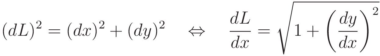
To prepare for later use: from midpoint to cusp the slope of the curve increases; the length of chain per unit of x-coordinate increases accordingly. (1.1) gives an expression for dL/dx.

$(dL)^2=(dx)^2+(dy)^2 \quad \Leftrightarrow \quad \frac{dL}{dx} = \sqrt{1 + \left(\frac{dy}{dx}\right)^2}$

(1.1)

In graphlet 2: as you move the slider you see that the force component in the horizontal direction is the same everywhere along the curve. The reason for that is the following: gravity is acting in the vertical direction, and there is only a single location where that force is redirected: at the cusp. To redirect a force that is transmitted by a flexible cable the cable must run over some sort of pulley. But from cusp to cusp there is no such pulley, therefore the horizontal tension component is the same along the length of the catenary.

The equilibrium shape has the following property: at every point along the length of the chain the tension force is tangent to the local slope.

At every point, from the mid point to the cusp, the chain above that point is providing the required force to support the weight of the length of chain below that point.

It follows: at every point along the curve: the slope of the curve (the tangent) coincides with the ratio of horizontal tension component and vertical tension component:

$\frac{dy}{dx} = \frac{\lambda L}{T_H}$

(1.2)

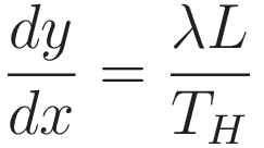
At this point the goal is to work towards an expression that is purely in terms of the cartesian coordinates x and y. (1.1) will get us there, but it gives an expression in terms of the derivative of L with respect to x, so in order to make use of (1.1) we need to take the derivative of (1.2) with respect to x.

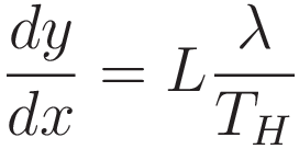
We take advantage of the fact that the horizontal tension component is not a function of the x-coordinate. We separate L from λ/T_H.

$\frac{dy}{dx} = L \frac{\lambda}{T_H}$

(1.3)

We take the derivative with respect to x:

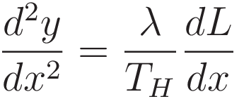
$\frac{d^2y}{dx^2} = \frac{\lambda}{T_H} \frac{dL}{dx}$

(1.4)

Combining (1.4) and (1.1) achieves the goal of converting the quantity dL: (1.5) is in terms of the cartesian coordinates x and y only:

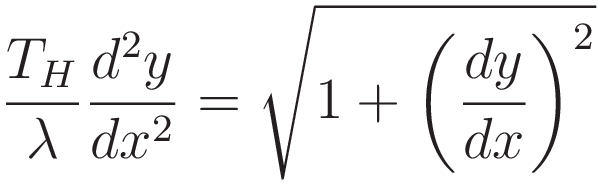
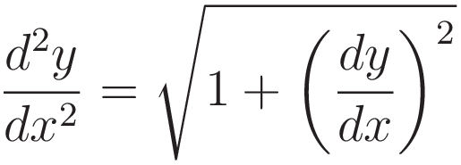
$\frac{T_H}{\lambda}\frac{d^2y}{dx^2} = \sqrt{1 + \left(\frac{dy}{dx}\right)^2}$

(1.5)

Given the form of the right hand side of (1.5) it is clear that if the differential equation has a solution at all it must involve the hyperbolic cosine; the sinh and cosh are related according to the equation: sinh²+1=cosh²

(It is in fact possible to work (1.5) down to a simpler expression, see Appendix I)

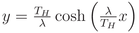
(1.6) incorporates the ratio T_H/λ such that it satisfies (1.5)

$y = \tfrac{T_H}{\lambda} \cosh \left(\tfrac{\lambda}{T_H} x \right)$

(1.6)

Statics, general nature of variational approach

Before discussing the proces of using calculus of variations to find the shape of the catenary I first want to discuss the nature of variational approach in general. To do that I start with the simplest case that admits representation in variational form. Graphlet 3. simplifies from the catenary problem to finding a force equilibrium of three equal weights.

Picture 3. Graphlet
Force equilibrium

I will refer to the weight in the center as 'the center weight'. I will refer to the two outer weights as if they constitute a single counterweight: 'the counterweight'. Each weight is 1 unit of mass.

Moving the slider sweeps out variation. The lower bound of the slider value puts the counterweight at the lowest possible position, given the length of the wire. The position of the counterweight follows the slider value. (For the upper bound of the slider the value of 0.3 was chosen because that is about twice the value of the slider at the equilibrium point.)

The wire, in the graphlet displayed as dashed lines, is treated as having negligable mass, so the force balance is determined by the positions of the weights only. With the checkbox 'force comparison' checked two arcs are displayed. When sweeping out variation: one arc is stationary, the other moves in response to variation. The stationary arc represents the magnitude of the force exerted by the counterweight. The dynamic arc represents the force in the wire as a function of the height of the center weight.

Potential energy

The variational approach evaluates rate of change of potential energy.

We have that when a mass m, subject to a gravitational force g descends over a height h the amount of gravitational potential energy that is released is mgh

Here the value of m is set to 1 unit of mass. The value of the gravitational acceleration g will drop out of the evaluation anyway, so for simplicity I treat the calculation for the case of g=1. Therefore the value of the potential energy E_p is the same as the value h for the height of the weight.

Picture 4. Graphlet
Left side: force comparison
Right side: potential energy comparison

In graphlet 3: in the right hand side subpanel the line with the long dashes gives the resultant potential energy.

As the counterweight rises the center weight descends. The intersection point of the center weight curve and the vertical slider value line follows the actual height of the center weight.

Picture 5. Diagram

F_t	Total force
F_v	Vertical component of the force
F_h	Horizontal component of the force (omitted from the diagram)
α	The angle of the wire with respect to the horizontal

Force calculation

To find the equilibrium angle:

Each of the two wires, to the left and to the right, carries half of the weight of the center weight, therefore the magnitude of the vertical force component is half a unit of force. The total force in each single wire is 1 unit of force.

Since the triangle is a right-angled triangle we have two calculation strategies available: Pythagoras' theorem and trigonometry. In this case using trigonometr is the quickest; but for the purpose of comparison with the potential energy evaluation I will use Pythagoras' theorem.

The total force as the resultant of the vertical force component and the horizontal force component:

(2.1)

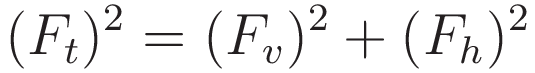
Rearranging gives an expression for the value of F_h in terms of F_t and F_v

$(F_h)^2 = \sqrt{(F_t)^2 - (F_v)^2}$

(2.2)

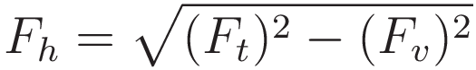
With F_t 1 unit of force and F_v half a unit of force:

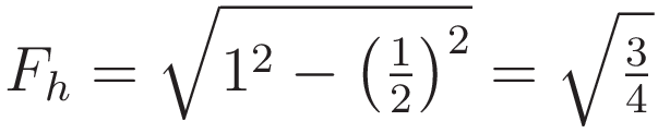
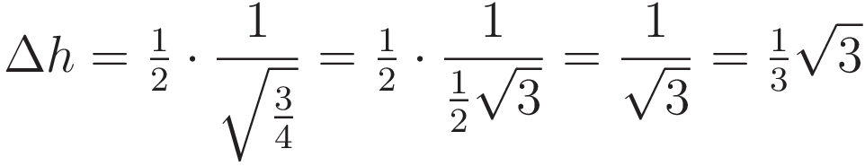
$F_h = \sqrt{1^2 - \left(\tfrac{1}{2}\right)^2} = \sqrt{\tfrac{3}{4}}$

(2.3)

To obtain the height of the centerweight where there is force equilibrium:
In the diagram the distance from the cusp to the center line is 1 unit of distance, and the horizontal force component is the square root of 3/4. So that is a ratio of √(3/4) The height difference Δh and the value of the vertical force component are in the same ratio to each other:

$\Delta h = \tfrac{1}{2} \cdot \frac{1}{\sqrt{\tfrac{3}{4}}} = \tfrac{1}{2} \cdot \frac{1}{\tfrac{1}{2}\sqrt{3}} = \frac{1}{\sqrt{3}} = \tfrac{1}{3}\sqrt{3}$

(2.4)

Here is how the value of the height difference is obtained with trigonometry:
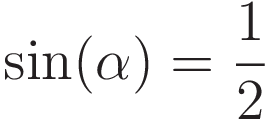
The sine of angle α is equal to F_v divided by F_t. That ratio is one half, hence the equilibrium angle is 30 degrees.

We obtain the equilibrium height from the angle: the distance from the center line to the cusp is 1 unit of distance, and the tangent of 30 degrees is 1/√3.

Potential energy evaluation

In order for a state of equilibrium to have meaning the system must have freedom to move. In the general case we assume there is freedom to move, either by way of parts sliding along each other, or by way of elastic deformation.

In the case depicted in Graphlet 3., the three weights: if the motion of the wire sliding over the cusps is low friction the system will tend to oscillate back and forth over the equilibrium point. Each time the system overshoots the equilibrium the direction of the resultant force reverses. The reversal is a reversal of direction of doing net work.

About doing work and doing negative work:
The concept of doing negative work is useful in situations where more than one force is being exerted, with the forces involved acting in opposite direction.

Example: the case of operating a crane: difference between lifting and lowering a load. When a load is being lifted the crane engine is doing positive work, and the force of gravity is doing negative work. Conversely, when the crane is lowering a load the engine is doing negative work, and gravity is doing positive work.

In the three weights case as represented with graphlet 2: the equilibrium point is the specific point where in both directions of motion each of the opposite forces is doing work at the same rate.

In the graphlet the height above zero of the counterweight is equal to the slider value. The total counterweight mass is two units of mass, therefore the rate of change of potential energy is two units of energy per unit of height.

Next: an expression for the center weight potential energy as a function of the slider value.

To make the expression a bit simpler I define an auxillary variable q. q is the total length of the hypotenuse. (With p for the slider value: q = p + 1)

Pythagoras' theorem then gives the following expression for the height h of the center weight as a function of q:

$h(q) = \sqrt{q^2 - 1}$

(2.5)

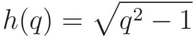
(As stated earlier: m is taken as 1 unit of mass, and g for gravity drops out anyway, so the value h for the height is the value of the Potential energy.)

The variation is variation of height. We obtain the rate of change of potential energy by taking the derivative of (2.5) with respect to the variational parameter.

$\frac{dh}{dq} = \frac{q}{\sqrt{q^2 - 1}}$

(2.6)

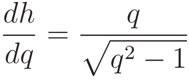
At this point we take advantage of the following: q, the value of the numerator of the right hand side of (2.6), is the length of the hypotenuse, and the value of the denominator is the length of the opposing side of angle α. Therefore we can use trigonometry; the inverse of the right hand side of (2.6) gives the sine of the angle α.

(2.7)

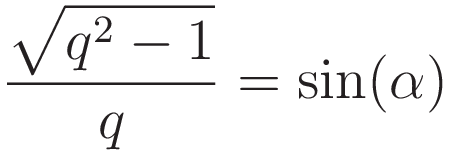
In order to do work at the same rate as the counterweights: the point where the center weight descends/ascends twice as fast as the counterweight is the equilibrium point. Therefore:

(2.8)

Integration and differentiation

As we know: integration and differentiation are each the inverse of the other (the integration up to an arbitrary constant.)

The potential energy is defined as the negative of work done, and work done is the integral of force over distance.

To find the point in the variation space where in both directions of motion the same amount of work is done we take the derivative of the potential energy with respect to the displacement.

The point is: taking the derivative of the potential energy with respect to the displacement is the reverse operation of the integration: after taking the derivative the evaluation is force evaluation.

(2.6) is stated in terms of the variational parameter q. This has the effect of scaling the right-angled triangle. The outcome of the evaluation is the same either way; the angle α is defined by the ratio of the opposing side and the hypotenuse.

The catenary, potential energy

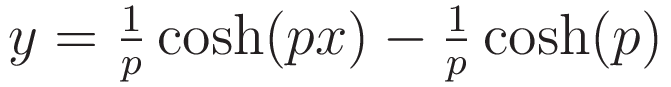
The value of the slider is used as variational parameter. I will refer to that value as p. In the graphlet the shape of the chain as a function of parameter p is implemented as follows:

$y = \tfrac{1}{p} \cosh(p x)$

(3.1)

More specifically: to make the cusps come out at y=0 the height of the cusps as a function of the variational parameter is subtracted.

$y = \tfrac{1}{p} \cosh(p x) - \tfrac{1}{p} \cosh(p)$

(3.2)

Graphlet 6.: the right side sub-panel displays the rate of change of the potential as a function of the value of the variational parameter. I will abbreviate 'rate of change of potentential as function of p' to: potential-change-rate

The graph for the potential-change-rate of the catenary section is overall below the graph for the potential-change-rate of the tensioning section.

The tensioning section and the catenary section are in counter-motion; when the catenary section descends the tensioning section moves upwards. In this diagram the potential-change-rate of the tensioning section has been mirrored in the x-axis. The mirroring of the graph allows direct comparison.

Picture 6. Graphlet
Catenary, rate of change of potential energy

Graphlet 7. displays the difference between the two change-rates. For clarity: in the right side sub-panel the vertical scaling has been increased by a factor of 10

Picture 7. Graphlet
Catenary, potential energy

The line with long dashes displays the difference between the two change-rates.

The line with the short dashes displays the integral. This integral is the resultant potential as a function of the variational parameter.

Appendix: simplifying the equation by differentiating

(I learned the following approach from Daniel Rubin. Youtube video: the Catenary )

(4.1) is (1.5) with the factor T_H/λ omitted.

(4.1)

We make the substitution , and we square both sides. Squaring both sides introduces an extraneous solution, so at a later stage we must discard that.

(4.2)

Next we take the derivative with respect to x:

(4.3)

Dividing both sides by 2du/dx:

(4.4)

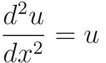
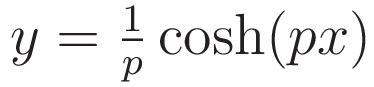
So the solution to the equation is a function with the property that if you differentiate it twice you get the same function back. That narrows the options down to the following two expressions:

(4.5)

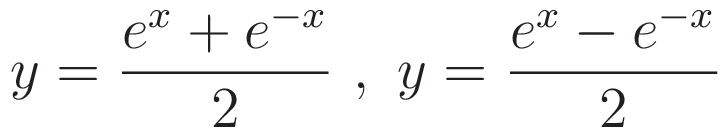
Of these two the first one satisfies (4.1)

Back to article

This work is licensed under a Creative Commons Attribution-ShareAlike 3.0 Unported License.

Last time this page was modified: April 22 2023